4.1 Escape Local Minimas?
We saw in the previous post that the overall potential function consists of multiple local minimas. One way to avoid is by using Randomized Path Planner (RPP). In this, series of random walks are initiated when the robot is stuck in the local minima. Another way can be using Navigation Potential Function which consists of only one minima which is at $q_{goal}$. This post will be focussed on Navigation Potential Function. More info about RRP can be found here
Before moving on further, lets discuss about Hessian matrix. Suppose a potential function $\nabla U(q)$ has a critical point at $q^{\dagger}$ i.e $\nabla U(q^{\dagger}) = 0$. The point $q^{\dagger}$ is either maximum, minimum or saddle point(Figure 4.1).One can look at the second derivative to determine the type of critical point. For real-valued functions, this second derivative is the Hessian matrix.
$$\left[ \begin{matrix} \frac{\partial^{2}U}{dq^{2}_{1}} & \cdots & \frac{\partial^{2}U}{\partial q_{1} \partial q_{n}} \\ \vdots & \ddots & \vdots \\ \frac{\partial^{2}U}{\partial q_{n} \partial q_{1}} & \cdots & \frac{\partial^{2}U}{dq^{2}_{n}} \\ \end{matrix} \right]$$
When the Hessian matrix is
- non-singular, then $q^{\dagger}$ is non-degenerate(isolated).
- positive-definite, then $q^{\dagger}$ is local minimum.
- negative-definite, then $q^{\dagger}$ is local maximum.
One can refer this wiki for matrix properties.
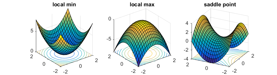
Figure 4.1 Minimum, Maximum, Saddle
4.2 Navigation Potential Function
As stated above, navigation potential function have one local minima. The formal definition is as follows:
A function $\varphi$ : $Q_{free} \to [0,1]$ is called navigation potential if it
- is smooth (or atleast $C^{k}$ for $k \geqslant 2$ continous derivatives)
- has unique minimum at $q_{goal}$ in the connected component of free space that contains $q_{goal}$
- is uniform maximal on the boundary of the free space
- is Morse
A morse function is one whose critical point($\frac{d}{dx}f(x) = 0$) are all non-degenrate i.e they are isolated.
4.3 Sphere Space
This approach intially assumes that the configuration space is bounded by a sphere centered at $q_{0}$ and has n $dim(Q_{free})$-dimensional spherical obstacles centered at $q_{1},q_{2},….q_{n}$. The spheres are assumed to be disjoint. The repulsive function is defined as
$\beta_{0}(q) = -d^{2}(q,q_{0}) + r^{2}_{0} \tag{1}$
$\beta_{i}(q) = d^{2}(q,q_{i}) - r^{2}_{i} \tag{2}$
where $r_{i}$ is the radius of $i^{th}$ sphere.
The overall repulsive function is written as the multiplication of every sphere,
${\displaystyle \prod_{i=0}^{n} \beta_{i}(q)} \tag{3}$
The repulsive function of $i^{th}$ sphere at the boundary is zero, positive inside the boundary and negative outside the boundary. However, for the $0^{th}$ it is positive outside the boundary and negative inside the boundary. We can think of a disc of some thickness removed from a solid block. Now, imagine a robot is kept in that empty space or impression indicating the configuration space the robot has to work in. Next, the attractive function is defined as
$\gamma_{k} = (d(q,q_{goal}))^{2k} \tag{4}$
where $k$ is a positive number.
Key Points:
-
the value of $\gamma_{k}$ is zero at goal.
-
$\frac{\gamma_{k}}{\beta}$ tends to $\infty$ as $q$ approaches boundary of an obstacle.
-
For large value of $k$, $\frac{\gamma_{k}}{\beta}$ has a unique minimum. As gradient $\frac{\partial \gamma_{k}}{\partial q}$ dominates $\frac{\partial \beta}{\partial q}$.
-
increasing the value of $k$ causes other minimas to gravitate towards boundary of the obstacle and the range of repulsive influence of obstacle becomes small relative to attractive fucntion.
-
only the nearby obstacle will have significant effect on value of $\frac{\gamma_{k}}{\beta}$.
-
therefore, only opportunity of local minima appear on the radial line of obstacle and goal.(One may refer to Figure 3.7 in previous post)
-
for a very large value of $k$, Hessian matrix can be positive definite. Therefore, only one minima can be at goal which is infact the global minima.
Now, we need to do some scaling as $\frac{\gamma_{k}}{\beta}$ can have any arbitary values. The following equation is called an analytical switch.
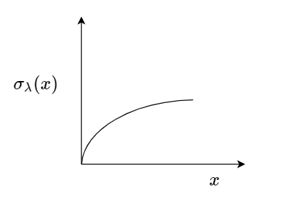
Figure 4.2 Analytical Switch
$\sigma_{\lambda}(x) = \frac{x}{\lambda + x} \tag{5}$
Lets see how this switch limits a given function. Take an example of $y = x^{2} $ and observe the Figure 4.3. Note: It is not scaled to graph.

Figure 4.3 Analytical switch limiting the function
We can now apply the same on the function $\frac{\gamma_{k}}{\beta}$. The function $s(q,\lambda)$ has a zero value at goal, unitary at boundary of an obstacle, and varies continuously in free space.
$s(q,\lambda) = (\sigma_{\lambda} \circ \frac{\gamma_{k}}{\beta})(q) = \frac{\gamma_{k}}{\lambda \beta + \gamma_{k}}(q) \tag{6}$
It has a unique minimum at for a large enough value of $k$. However, this is still not necessarily a Morse function. So, we introduce another function to sharpen $s(q,\lambda)$. This sharpening function is
$\xi_{k} = x^\frac{1}{k} \tag{7}$
$\varphi(q) = (\xi_{k} \circ \sigma_{\lambda} \circ \frac{\gamma_{k}}{\beta})(q) = \frac{d^2(q,q_{goal})}{[(d(q,q_{goal}))^{2k} + \lambda \beta(q)]^\frac{1}{k}} \tag{8}$
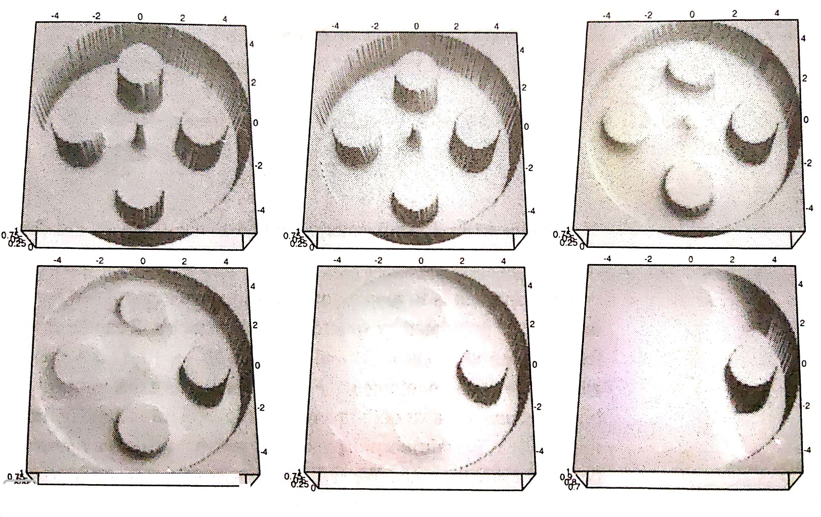
Figure 4.4 Visualization of navigation function with five obstacles for $k=3,4,5,6,7,8,10$
The effect of increasing $k$ can be seen in the Figure 4.4. For $k=10$, $\varphi$ has one minima which is at goal.
4.4 Implementation
Similar to our previous post, the velocity can be considered as gradient of this function. Before that, we need to determine the value of $\lambda$. The value of $\lambda$ should be such that,
$\frac{\lambda \beta}{\gamma_{k}} << 1. \tag{9}$
The value of $\gamma_{k}$ will be maximum on the boundary point $\dagger$ with its line segment to goal passing through the center of $0^{th}$ obstacle. With the same boundary point $\dagger$, we can further calculate the value of $\beta(q)$. Finally, the value of $\lambda$ can be calculated as,
$ \lambda = |\frac{\beta^{\dagger}}{\gamma^{\dagger}_{k}}| \epsilon \tag{10}$
$where, \epsilon = 1e-25$
The value of $\epsilon$ was experimentally determined by analysing the strength of repulsive potential against the attractive potential.
4.5 Conclusion
The main takeaways of this function is-
- It can be extended to higher dimensions as well.
- It has only one local minimum which is at $q_{goal}$.
- Though it has only one local minimum, it suffers from saddle points which results in wobbly motion of the robot.
- One may observe in Figure 4.4 for $k=10$, the magnitude of the function is almost constant everywhere resulting in steep changes near the goal.
</> GitHub
4.6 References
[1]. Choset H., Lynch K. M., Hutchinson S. Kantor G., Burgard W., Kavraki L. E., Thrun Sebastian. Principles of Robot Motion. MIT Press
[2]. RI16-735 Robot Motion Planning - link