7.1 Recall!
From the previous post, we learned that \(f(n) = h(n)\) search becomes greedy and \(f(n) = g(n)\) search grows path that is shortest from start until it encounters the goal(Dijkstra’s algorithm or Uninformed A*). Now, the A* algorithm is just the combination of both.
$$f(n) = h(n) + g(n) \tag{1}$$
Now, lets take a deeper dive in the algorithm.
7.2 A* Algorithm
I bet you remember all the terminologies.
Now, take a pen and a scratch paper and try to understand the algorithm by solving the following example. Assume the function $h(s)$ gives the number of nodes $s$ is away from $s_{goal}$ and $g(s) = g(s_{start}) + c(s_{start},s)$, where $c$ is the edge cost. So, $h(s_{goal}) = 0$ and $g(s_{start}) = 0$. Try it out on your own and compare it with the below table.

Figure 7.1 Example
Table 1 Solution
| Node To Expand | OPEN | CLOSED | bp(s) |
|---|---|---|---|
| $s_{start}$ | {$s_{start}$} | {} | - |
| $s_2$ | {$s_2$} | {$s_{start}$} | $bp(s_2) = s_{start}$ |
| $s_4$ | {$s_4, s_1$} | {$s_{start}, s_2$} | $bp(s_4) = bp(s_1) = s_2$ |
| $s_1$ | {$s_3, s_1$} | {$s_{start}, s_2, s_4$} | $bp(s_3) = s_4$ |
| $s_{goal}$ | {$s_3, s_{goal}$} | {$s_{start}, s_2, s_4, s_1$} | $bp(s_{goal}) = s_1$ |
| - | {$s_3$} | {$s_{start}, s_2, s_4, s_1, s_{goal}$} | - |
Finally, in order to find the least cost path, we have to just follow the backpointers all the way from $s_{goal}$ to $s_{start}$. So, in our case the path will be $s_{goal} \rightarrow s_1 \rightarrow s_2 \rightarrow s_{start}$.
7.3 Weighted A*
The name itself suggests that some weight or priority is assigned to the function.
$f(s) = g(s) + \epsilon h(s) \tag{2}$
For $\epsilon \geq 1$, there is a bias towards nodes that are closer to goal. We may regard weighted A* as greedy for a very high value of $\epsilon$. If we allow an epsilon of 5, this means that the weighted A* algorithm will return a path that is no worse than 5 times the cost of the optimal solution.
7.4 Backward A*
It is similar to conventional A* algorithm, but the difference is that one starts to search from goal to the start. Accordingly, the algorithm changes to
7.5 Conclusion
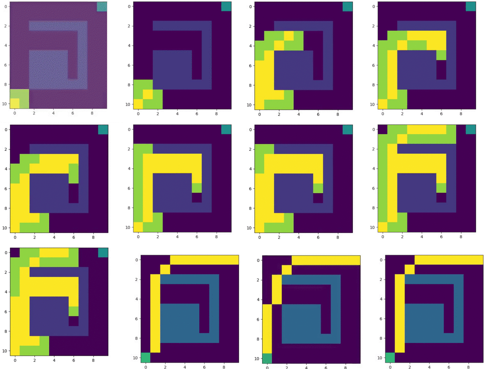
The major difference between A* and weighted A* is the tradeoff between optimal solution and computation time. In following figure, two scenarios are taken: $\epsilon = 1$ and $\epsilon = 2.5$

Figure 7.2 A* $\epsilon = 1$ vs $\epsilon = 2.5$
Here, green indicates OPEN states and yellow indicates CLOSED states. The weighted A* is able to find solution faster than A*. However, the solution given by weighted A* is sub-optimal.
</> GitHub
7.6 References
[1]. 16-350 Planning Techniques for Robotics - link
[2]. Online - http://sbpl.net/

