3.1 Basic Idea
Potential function approach directs a robot as if it were a particle moving in a gradient vector field. Gradients can be viewed as forces acting on a positively charged particle robot attracted by a negatively charged goal. Obstacles are also positively charged which forms a repulsive force directing the robot away from it.
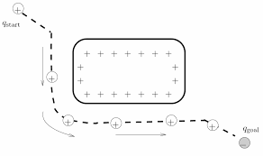
Figure 3.1 -ve goal attarcts +ve robot
A potential function can be constructed as a sum of attractive and repulsive potenials.
$U(q) = U_{att}(q) + U_{rep}(q) \tag{1}$
We will consider the gradient of the potential function as a velocity vector($\vec{v}$).
$v = -\nabla U(q) \tag{2}$
Note: The function must be continuously differentiable.
3.2 Attractive Potential
The simplest attractive potential function is one that grows quadratically with the distance to goal. Let $\zeta$ be a parameter used to scale the effect of the attractive potential function and $d(q,q_{goal})$ be the distance from current configuration $q$ to goal configuration $q_{goal}$.
$U_{att}(q) = \frac{1}{2}\zeta d^{2}(q,q_{goal}) \tag{3}$
In Figure 3.2, we can observe that as we move closer towards the goal the energy decreases and becomes zero at the goal(global minimum).
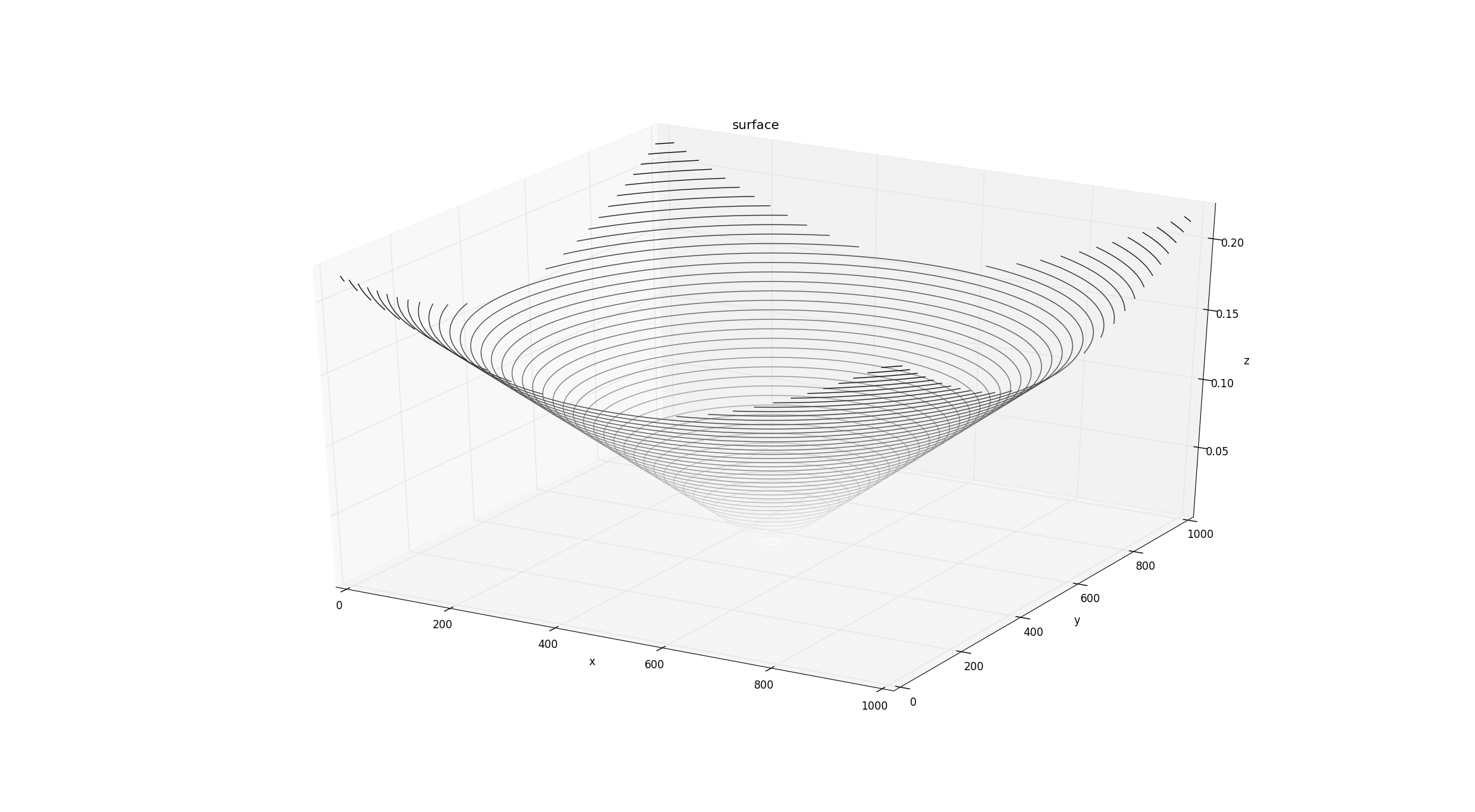
Figure 3.2 Attractive Potential Function $goal: (500,500)$
As discussed in the earlier post that our robot can move only in plane. From eqn(2), we can write
$\vec{v} = -\nabla U(q) = \zeta (x_{g}-x) \hat{i} + \zeta (y_{g}-y) \hat{j}. \tag{4}$
The argument $\theta$ of the vector can be given by
$\theta = atan2(y_{g}-y,x_{g}-x). \tag{5}$
The magnitude of the vector can be given by
$|v| = \zeta \sqrt{(x_{g}-x)^{2} + (y_{g}-y)^{2}} \tag{6}$ $or$ $|v| = \zeta d^{2}(q,q_{goal}). \tag{7}$
We can find the value of $\zeta$ by subsituting the $|v|$ as maximum linear velocity of robot and $d(q,q_{goal})$ as the distance from start configuration $q_{start}$ to the goal configuration $q_{goal}$. Therefore,
$\zeta = \frac{|v_{max}|}{d^{2}(q_{start},q_{goal})}. \tag{8}$
3.3 Repulsive Potential
The repulsive potential keeps the robot away from the obstacles. It is usually defined in terms of how close the robot is to the obstacle. Here, we will only consider the effect of the nearest obstacle. Let $D(q)$ be the distance from the robot's current position $(x,y)$ to the nearest point $(x_{o},y_{o})$ on obstacle and $Q^{\dagger}$ be the tolerance which allows the robot to ignore the obstacle. The function is defined as
$U_{rep}(q) = \begin{cases} \frac{\eta}{2} (\frac{1}{D(q)} - \frac{1}{Q^{\dagger}})^{2}, & \text{$D(q) \leqslant Q^{\dagger}$} \\ 0, & \text{$D(q) > Q^{\dagger}$} \tag{9} \end{cases} $
The following graph shows potential energy of two cylindrical obstacles of radius = $20cm$ and $Q^{\dagger}$ = $30cm$. 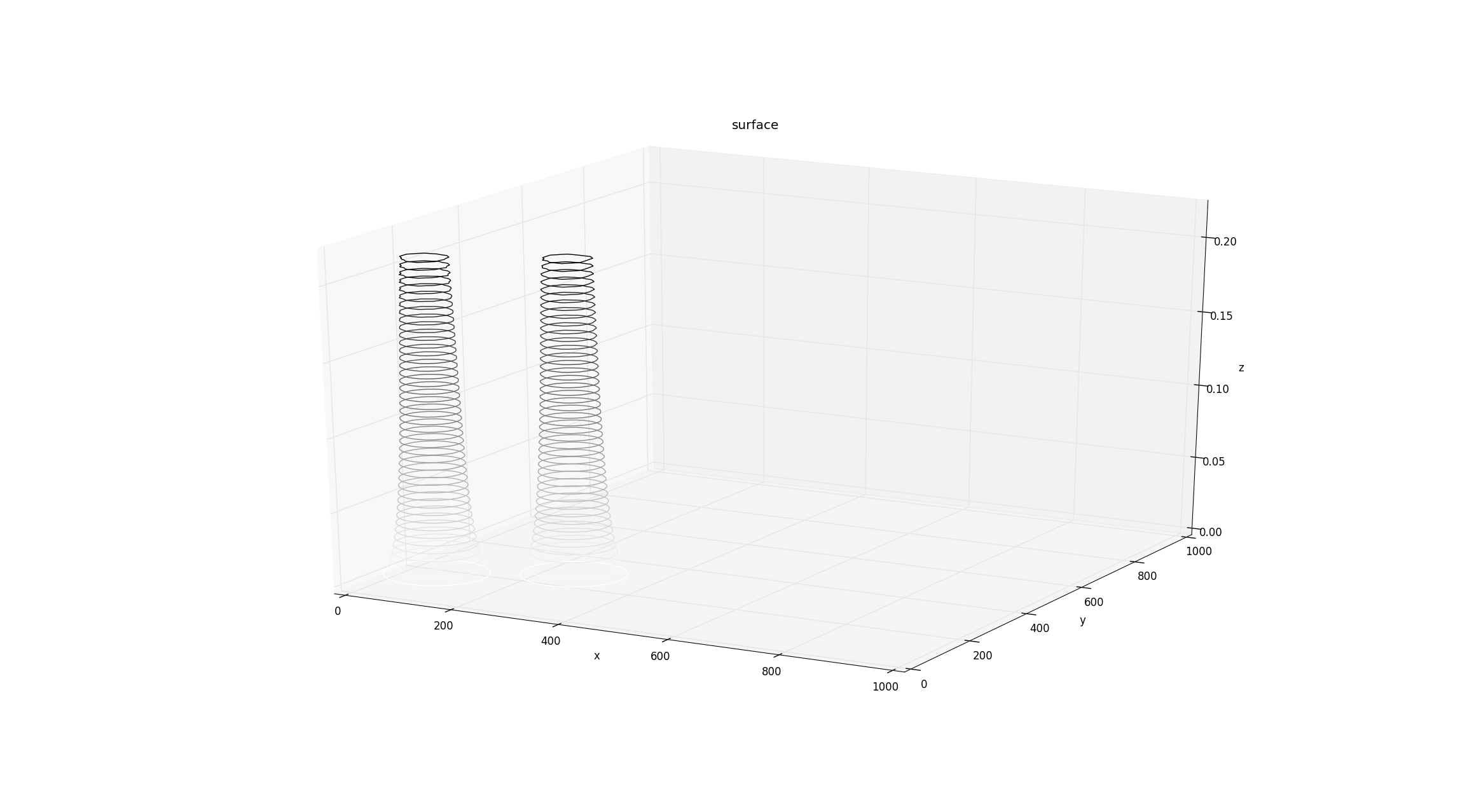
Figure 3.3 Repulsive Potential Function - two cylindrical obstacles
Also, the velocity vector is given by
$\vec{v} = - \nabla U_{rep}(q) = \begin{cases} - \eta (\frac{1}{D(q)} - \frac{1}{Q^{\dagger}}) \frac{1}{D^{2}(q)} \nabla D(q), & \text{$D(q) \leqslant Q^{\dagger}$} \\ 0, & \text{$D(q) > Q^{\dagger}$} \tag{10} \end{cases} $
$where, \nabla D(q) = \frac{(x_{o}-x)^{2}}{D(q)} \hat{i} + \frac{(y_{o}-y)^{2}}{D(q)} \hat{j} \tag{11} $
Similar to eqn(5) the argument $\phi$ is given by
$\phi = atan2(y - y_{o},x - x_{o}). \tag{12}$
One should be very careful while calculating the argument of the vector as we require an angle from point $D(x_{o},y_{o})$ to point $P(x,y)$. **Figure 3.4** should make this more clear. _Note: atan2 gives quadrant specific angles_
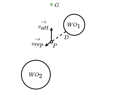
Figure 3.4 Only nearest obstacle is considered
Similar to eqn(6) the magnitude is given by
$|v| = |\eta (\frac{1}{Q^\dagger} - \frac{1}{D(q)}) \frac{1}{D^{2}(q)} \nabla D(q)|. \tag{13}$
$\because |\nabla D(q)| = 1 \tag{14}$
$|v| = |\eta (\frac{1}{Q^\dagger} - \frac{1}{D(q)}) \frac{1}{D^{2}(q)}| \tag{15}$
Now, the value of $\eta$ can be calculated when $D(q)$ is minimum. One may think $D(q)$ to be zero which is not practically possible as the $360^{\circ}$ LIDAR or any other sensor has some minimum and maximum value. For our case, the minimum distance the laser can sense is $0.12m$. Plugging the value of $D(q)$ as $0.12m$ and $|v|$ as $|v_{max}|$, we can calculate the value of $\eta$.
From Figure 3.5, we can now observe the overall potential function $U(q)$. 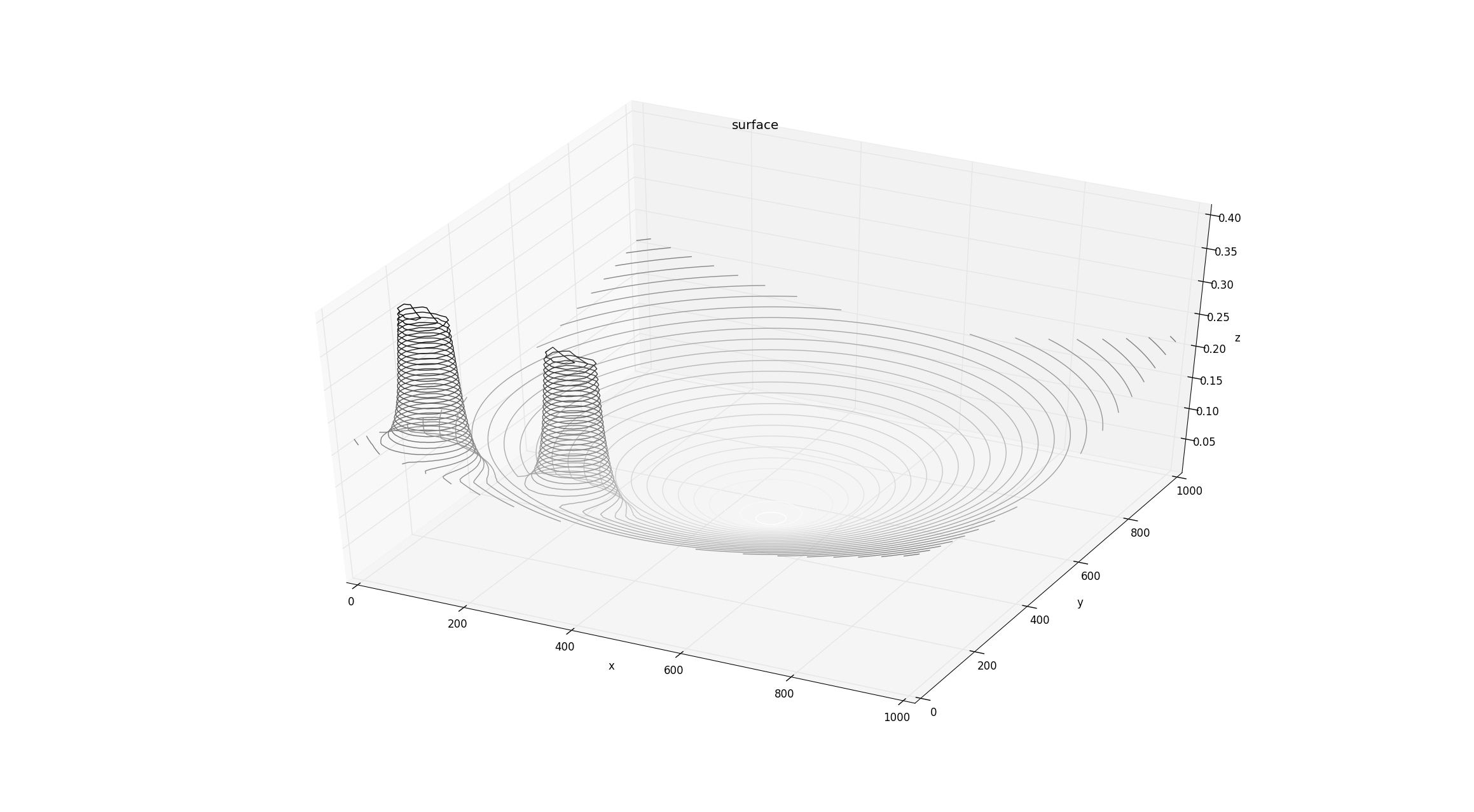
Figure 3.5 Potential Function (Att + Rep)
3.4 Results
Figure 3.6 is the simulation result with following environment configuration:
- Start = $S(0,0)$
- Goal = $G(500,500)$
- Cylindrical obstacle at $(100,130)$ and $(330,270)$ with raidus of $10cm$
- Reference point used to construct the configuration space obstacles is center of the robot
- $Q^{\dagger} = 30cm$
Note: The robot can reach the goal with any orientation 
Figure 3.6 Results
Video:
One might have observed in the video that the robot struggled to move when it was near the second obstacle.
3.5 The Local Minima Problem
**Figure 3.7** illustrates the condition which might have occured in the simulation test. We can see the repulsive velocity acting in the direction opposite to the attractive velocity. Resulting in only decrease in the magnitude of the resultant vector.
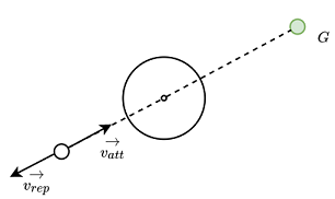
Figure 3.7 One obstacle creating a local minima
Figure 3.8 illustrates a condition when all the obstacles in range(sensors) are considered and accordingly repulsive vectors are generated.
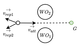
Figure 3.8 Two obstacles creating a local minima
These are some of the drawbacks of potential functions. We can conclude that potential function is not **complete**. In the next post, we will se how can we avoid the local minimas. However, potential functions are known for their generalization to higher dimensions too.
</> GitHub
3.6 References
[1]. Choset H., Lynch K. M., Hutchinson S. Kantor G., Burgard W., Kavraki L. E., Thrun Sebastian. Principles of Robot Motion. MIT Press
[2]. RI16-735 Robot Motion Planning - link
Bonus!
$U_{att} = \zeta d(q,q_{goal})$
Considering $\vec{v} = -\nabla U$,
- What will be the magnitude of the vector $\vec{v}$?
- What will be the argument of the vector $\vec{v}$?
- Is it feasible to use such attractive potential? Yes/No why?